What is Deep Learning and how does it work? Explained for beginners by Digimagg

What is Deep Learning?

Deep learning, a subset of machine learning, draws inspiration from the human brain's architecture. Its algorithms aim to mimic human-like reasoning by systematically analyzing data with predefined logical frameworks. This is facilitated by neural networks, which consist of layered algorithms.

Deep learning falls under the umbrella of machine learning, which, in turn, is a component of artificial intelligence. Artificial intelligence encompasses techniques enabling computers to emulate human behavior. Machine learning involves algorithms trained on data to achieve this. Deep learning, inspired by the human brain's structure, is a specific form of machine learning.

How does Deep Learning work?

Deep learning algorithms endeavor to derive comparable insights to human reasoning by continuously analyzing data structured in a specific manner. This is facilitated through the utilization of neural networks, which comprise multiple layers of algorithms.

The architecture of neural networks is inspired by the structure of the human brain. Just as humans utilize their brains to recognize patterns and categorize various types of information, neural networks can be trained to perform similar tasks on data.

Each layer within neural networks can be viewed as a filter that operates progressively from coarse to intricate, thereby enhancing the likelihood of producing accurate outcomes. This mirrors the functioning of the human brain, which compares incoming information with existing knowledge. Deep neural networks employ this same principle.

Neural networks enable a multitude of tasks such as clustering, classification, and regression. They can group or organize unlabeled data based on similarities among samples or categorize samples into different groups using labeled datasets.

In essence, neural networks can perform tasks akin to classical machine learning algorithms, but the reverse is not true. Artificial neural networks possess distinctive capabilities that allow deep learning models to tackle challenges beyond the reach of traditional machine learning models.

The significant strides in artificial intelligence witnessed in recent years are attributed to deep learning. Without it, advancements such as self-driving cars, chatbots, and virtual assistants like Alexa and Siri would not exist. Google Translate would remain rudimentary, and Netflix would lack personalized recommendations. Neural networks underpin all these deep learning applications and technologies.

An industrial revolution fueled by artificial neural networks and deep learning is underway. Ultimately, deep learning stands as the most effective and apparent avenue towards achieving true machine intelligence.

What makes Deep Learning so widely embraced?

No feature extraction

One primary benefit of deep learning compared to machine learning lies in the elimination of the need for manual feature extraction, also known as feature engineering.

Before the advent of deep learning, traditional machine learning techniques such as decision trees, SVM, naïve Bayes classifier, and logistic regression were commonly utilized. These algorithms, often referred to as "flat" algorithms, require a preprocessing step known as feature extraction before they can be applied directly to raw data such as .csv files, images, or text.

Feature extraction involves transforming the raw data into a representation that these classic machine learning algorithms can utilize to perform tasks such as classification into various categories or classes. This preprocessing step is typically intricate and necessitates a deep understanding of the problem domain. It requires adaptation, testing, and refinement over multiple iterations to achieve optimal results.

In contrast, deep learning's artificial neural networks bypass the need for feature extraction. The layers within these networks have the capability to autonomously learn an implicit representation of the raw data directly.

Here's the mechanism: Through multiple layers of an artificial neural network, a progressively abstract and condensed representation of the raw data is generated. This compressed representation of the input data is then employed to produce the desired outcome, such as the classification of input data into distinct classes.

In essence, the feature extraction process is inherently integrated into the operations of an artificial neural network.

Throughout the training phase, the neural network fine-tunes this process to derive the most optimal abstract representation of the input data. Consequently, deep learning models require minimal manual intervention to execute and refine the feature extraction procedure.

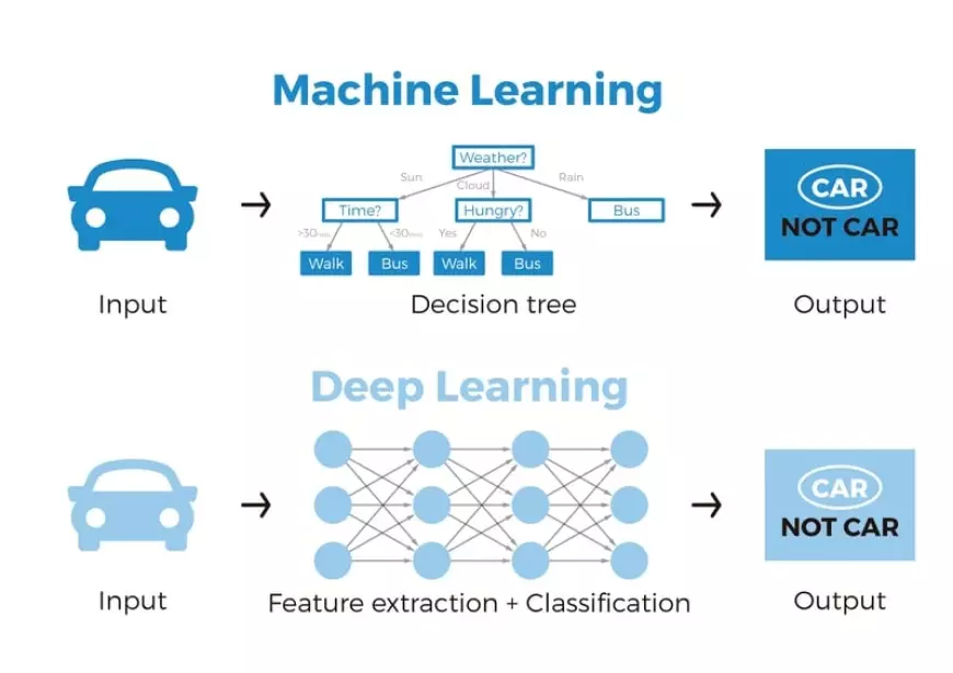
To illustrate, suppose we aim to employ a machine learning model to discern whether a given image depicts a car or not. Traditionally, humans must initially identify the distinct features of a car (such as shape, size, windows, wheels, etc.), extract these features, and provide them to the algorithm as input data. Subsequently, the algorithm performs image classification. Essentially, in machine learning, direct programmer intervention is essential for the model to reach a conclusion.

However, in the context of a deep learning model, the feature extraction step becomes obsolete. The model inherently recognizes these unique car characteristics and accurately predicts outcomes without human intervention.

In fact, abstaining from explicit feature extraction applies to every task performed with neural networks. Simply furnish the raw data to the neural network, and the model autonomously handles the rest.

Boosting Deep Learning accuracy with big data

Another significant advantage of deep learning, which underscores its growing popularity, is its reliance on vast quantities of data. The era of big data presents immense opportunities for innovation in deep learning. Andrew Ng, the chief scientist of Baidu, a prominent search engine in China, co-founder of Coursera, and a key figure in the Google Brain Project, aptly compares AI to building a rocket ship. He states:

"I think AI is akin to building a rocket ship. You need a huge engine and a lot of fuel. If you have a large engine and a tiny amount of fuel, you won’t make it to orbit. If you have a tiny engine and a ton of fuel, you can’t even lift off. To build a rocket you need a huge engine and a lot of fuel."

In the context of deep learning, the rocket engine symbolizes the deep learning models, while the fuel represents the vast amounts of data that can be input into these algorithms.

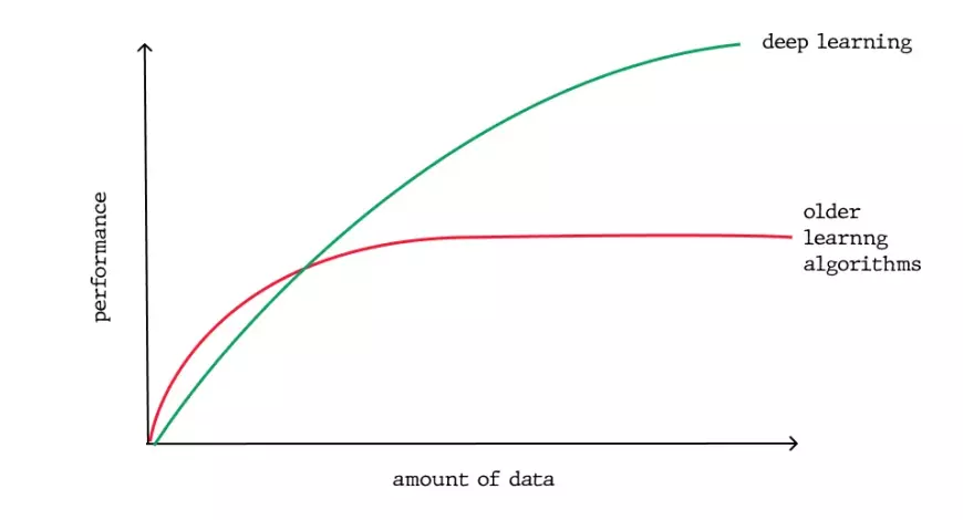
Deep learning models typically enhance their accuracy as they are trained with larger datasets, unlike traditional machine learning models like SVM and naive Bayes classifier, which plateau in improvement after reaching a saturation point.

How do Deep Learning neural networks work?

Artificial neural networks

Now that we have a fundamental grasp of the functioning of biological neural networks, let's delve into the structure of artificial neural networks.

An artificial neural network typically comprises interconnected units or nodes, referred to as neurons. These artificial neurons are inspired by the biological neurons found in our brain.

A neuron serves as a visual representation of a numerical value (e.g., 1.2, 5.0, 42.0, 0.25, etc.). In the context of a biological brain, any connection between two artificial neurons can be likened to an axon. These connections between neurons are established through weights, which are essentially numerical values.

During the learning process of an artificial neural network, these weights between neurons undergo adjustments, affecting the strength of connections. But what does this entail? When presented with training data and a specific task, such as classifying numbers, the objective is to determine a particular set of weights that enable the neural network to carry out the classification.

The set of weights varies for each task and dataset. Anticipating the precise values of these weights in advance is impractical; instead, the neural network must learn them. This process of acquiring knowledge is known as training.

Biological neural networks

Artificial neural networks draw inspiration from the structure of biological neurons present in the human brain. These artificial counterparts emulate certain fundamental aspects of biological neural networks, albeit in a simplified manner. To gain insights into artificial neural networks, it's beneficial to examine the structure of biological neural networks.

In essence, a biological neural network comprises a multitude of neurons.

Layer connections in a Deep Learning neural network

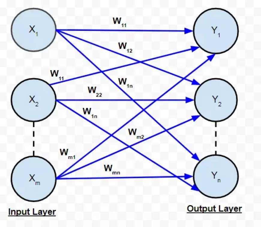
Let's consider a simplified neural network with just two layers. The input layer contains two neurons, and the output layer comprises three neurons.

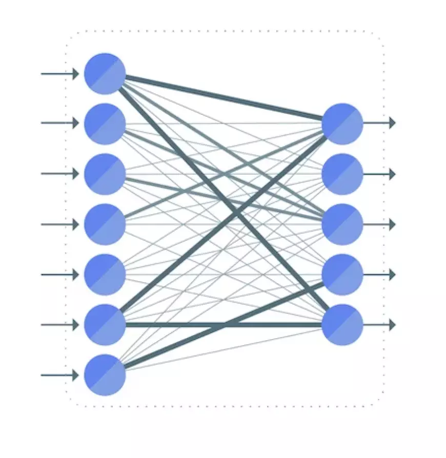
As previously discussed, the connection between two neurons is denoted by a numerical value known as a weight.

In the illustration, each connection between two neurons is associated with a distinct weight, represented by the symbol "w." These weights are indexed, with the first value indicating the number of neurons in the layer from which the connection originates, and the second value indicating the number of neurons in the layer to which the connection leads.

All the weights between layers of the neural network can be encapsulated in a matrix referred to as the weight matrix.

A weight matrix contains the same number of elements as the total connections between neurons. Its dimensions are determined by the sizes of the two layers linked by this matrix.

The number of rows aligns with the neurons' count in the layer from which the connections originate, while the number of columns aligns with the neurons' count in the layer to which the connections lead.

In this specific case, the weight matrix's rows correspond to the input layer's size, which is two, and its columns correspond to the output layer's size, which is three.

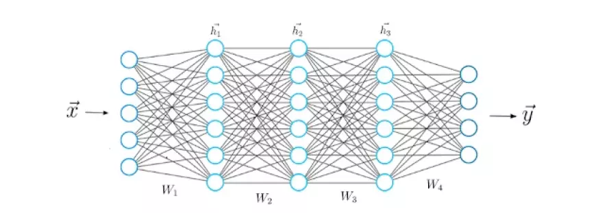
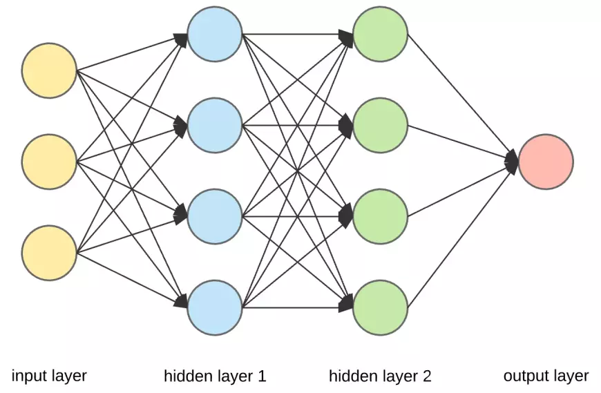
Deep Learning neural network architecture

In the standard neural network structure, there are multiple layers, with the initial one referred to as the input layer. This layer receives input, denoted as x, which comprises the data from which the neural network learns. For instance, in our earlier scenario of classifying handwritten numbers, these inputs x would correspond to the images of these numbers. Essentially, x is a complete vector where each entry represents a pixel.

The input layer contains the same number of neurons as there are elements in the vector x. Essentially, each input neuron corresponds to one element in the vector.

The final layer, known as the output layer, produces a vector y that represents the outcome of the neural network. Each entry within this vector corresponds to the activation values of the neurons in the output layer. In the context of classification tasks, each neuron in this final layer signifies a distinct class.

In this scenario, the activation value of an output neuron indicates the likelihood that the input features x, typically representing a handwritten digit, belong to a specific class (such as one of the digits 0-9). It's important to ensure that the number of output neurons matches the number of distinct classes.

To generate the prediction vector y, the network undergoes various mathematical operations within the hidden layers, situated between the input and output layers. These intermediary layers facilitate the transformation of input data into meaningful output predictions. Now, let's delve into the structure of connections between these layers.

Loss Functions in Deep Learning

Once the neural network generates its prediction, it's necessary to contrast this prediction vector with the actual ground truth label, denoted as y_hat. 

While the vector y represents the predictions computed by the neural network during forward propagation, which might diverge significantly from the true values, y_hat holds the actual values.

Mathematically, we gauge the disparity between y and y_hat by establishing a loss function, the magnitude of which hinges on this disparity.

An instance of a common loss function is the quadratic loss:

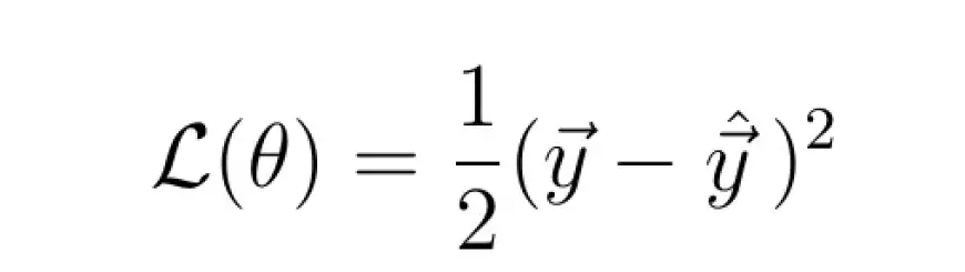
The magnitude of the loss function relies on the dissimilarity between y_hat and y. A greater difference results in a higher loss value, whereas a smaller difference yields a lower loss value.

Directly minimizing the loss function leads to enhanced accuracy in the neural network's predictions, as it reduces the disparity between the prediction and the actual label.

By minimizing the loss function, the neural network model automatically improves its predictive performance, irrespective of the specific characteristics of the task at hand. The key lies in selecting the appropriate loss function for the task.

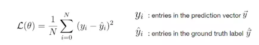
Thankfully, for most practical problems, just two primary loss functions are essential: the cross-entropy loss and the mean squared error (MSE) loss.

The cross-entropy loss

Mean squared error loss

Because the loss is influenced by the weights, it's necessary to discover a particular combination of weights that minimizes the loss function. This optimization process is accomplished mathematically using a technique known as gradient descent.

Learning a Deep Learning neural network’s process

With a clearer understanding of the neural network's structure, we can delve into the learning process systematically. Let's break it down step by step. The initial step, which you're already familiar with, involves the neural network computing a prediction vector, denoted as h, for a given input feature vector x.

This step is commonly referred to as forward propagation. It entails using the input vector x and the weight matrix W, which connects the two layers of neurons, to calculate the dot product between x and W. The outcome of this dot product is yet another vector, denoted as z.

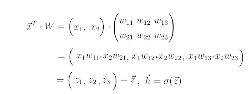
The final prediction vector, denoted as h, is obtained by applying an activation function, often denoted by the symbol sigma, to the vector z. This activation function serves as a nonlinear mapping from z to h.

In deep learning, there are three commonly used activation functions: tanh, sigmoid, and ReLU.

At this juncture, it becomes evident that neurons in a neural network simply represent numerical values. Let's take a closer examination of the vector z for a moment.

Each element of z comprises the input vector x. The significance of the weights becomes apparent here. The value of a neuron in a layer is a result of a linear combination of the values of neurons from the preceding layer, weighted by numeric values.

These numeric values represent the weights, indicating the strength of connections between neurons.

During training, these weights undergo adjustments, causing some neurons to become more strongly connected while others become less so. Similar to biological neural networks, learning in artificial neural networks involves altering weights. Consequently, the values of z, h, and the final output vector y fluctuate with the weights. Some weights bring the predictions of a neural network closer to the actual ground truth vector y_hat, while others increase the discrepancy.

Now equipped with an understanding of the mathematical operations between two neural network layers, we can expand our comprehension to encompass deeper architectures consisting of five layers.

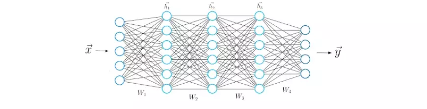
Similar to the previous step, we compute the dot product between the input vector x and the first weight matrix W1, and then apply an activation function to the resultant vector, yielding the first hidden vector, h1. We subsequently regard h1 as the input for the subsequent third layer. This process is iterated until we ultimately derive the final output vector, y.

Gradient descent in Deep Learning

In the process of gradient descent, we utilize the gradient of a loss function (essentially its derivative) to refine the weights of a neural network.

To grasp the fundamental idea behind gradient descent, let's examine a simple example of a neural network comprising just one input and one output neuron connected by a weight value, denoted as w.

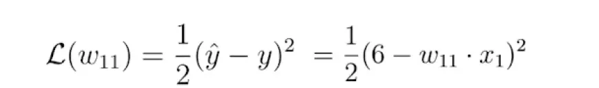
In this neural network, an input x is received, and a prediction y is generated as output. Suppose the initial weight value of this neural network is 5, and the input x is 2. Consequently, the prediction y of this network would be 10, while the label y_hat might be 6.

This indicates that the prediction is inaccurate, prompting us to employ the gradient descent method to determine a new weight value that enables the neural network to make the correct prediction. As a preliminary step, we need to select a suitable loss function for the task.

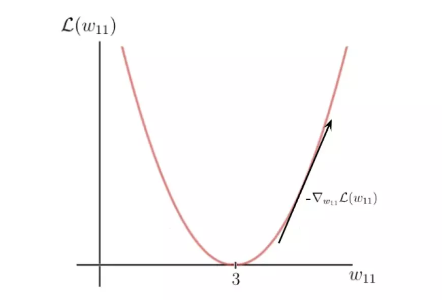
Let's opt for the quadratic loss function mentioned earlier and visualize this function, which essentially manifests as a quadratic function:

The y-axis denotes the loss value, which is contingent upon the disparity between the label and the prediction, and consequently, the network parameters — specifically, the single weight parameter, w, in this instance. On the other hand, the x-axis represents the range of values for this weight.

As evident, there exists a particular weight, denoted as w, at which the loss function attains a global minimum. This value represents the optimal weight parameter that would facilitate the neural network in making the correct prediction, which, in this scenario, is 6. Remarkably, the value for this optimal weight is identified as 3.

Conversely, our starting weight of 5 results in a relatively high loss. The objective now is to iteratively adjust the weight parameter until we converge upon the optimal value for that specific weight. This is where we employ the gradient of the loss function.

Fortunately, in this scenario, the loss function is solely a function of one variable: the weight, denoted as w.

Next, we compute the derivative of the loss function concerning this parameter:

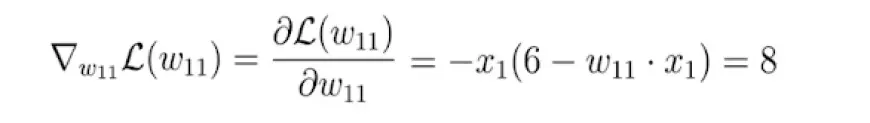
Ultimately, we obtain a value of 8, which represents the slope or tangent of the loss function at the corresponding point on the x-axis, where our initial weight resides.

This tangent indicates the direction of the steepest increase in the loss function and the corresponding weight parameters along the x-axis.

Essentially, by leveraging the gradient of the loss function, we've determined which weight parameters would lead to an even higher loss value. However, our objective is precisely the opposite. We can achieve this by multiplying the gradient by -1, thus obtaining the inverse direction of the gradient.

This process yields the direction of the highest rate of decrease in the loss function and the corresponding parameters along the x-axis that drive this reduction:

In the last step, we execute a single gradient descent iteration to refine our weights. Employing the negative gradient, we adjust our current weight in the direction that leads to a decrease in the loss function value, as dictated by the negative gradient:

The parameter epsilon in this equation represents a hyper-parameter known as the learning rate. It governs the pace at which we adjust the parameters during optimization.

It's important to note that the learning rate is the scalar value by which we scale the negative gradient, and typically, it is kept relatively small. In our case, the learning rate is set to 0.1.

As illustrated, after executing the gradient descent step, our weight w is now 4.2, bringing it closer to the optimal weight compared to its previous value.

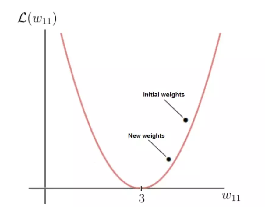
The reduced value of the loss function for the updated weight indicates an improvement, implying that the neural network is now more adept at making accurate predictions. By mentally performing the calculation, you'll observe that the new prediction is indeed closer to the label compared to before.

With each weight update, we descend along the negative gradient, progressively approaching the optimal weights. Following each gradient descent iteration, the network's current weights converge closer and closer to the optimal weights, ultimately enabling the neural network to make the desired predictions.